Who Needs Attention Anyway? Retaining State Corrections in Recurrent Control

Carrying a folding correction forward

The next proposal starts from the state you corrected.

Propose
Correct
Move
Next decision

Current chainProposed fold

Navigation: an agent crosses a maze with narrow doorways and moving circular obstacles to reach a goal.

Chain control: a 12-link articulated chain reaches three targets while avoiding obstacles, self-collision and joint limits.

Each decision receives a new observation, updates the hidden state and executes the first action of a short plan.

Evidence

Repeated derivative evaluations: ≈23%Fewer over the next eight decisions
Episode success gain: +2.7 / +4.4Percentage points · navigation / chain control
Network weights: FixedCorrections live in runtime memory

Paired tests in navigation and articulated chain control. Derivative evaluations count the task errors and derivatives computed during optimization.

We apply the same correction to two copies of the controller, keeping the corrected state in one and restoring the original state in the other. Over the next eight decisions, keeping the correction reduces repeated optimizer work. We count residual-Jacobian evaluations: computing the task errors and their derivatives for an optimization update.

Navigation: fewer evaluations: 23.1%
Chain control: fewer evaluations: 23.9%

Navigation uses 9.3 evaluations after retention versus 12.1 after discard; chain control uses 10.8 versus 14.2. Paired 95% intervals for the reductions are [17.0, 29.0]% and [17.5, 30.0]%.

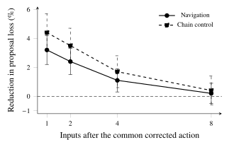
To measure the memory effect alone, we also disable further optimization and replay identical observations into both branches. Retaining the state lowers the next proposed plan's task loss by 3.2% in navigation and 4.4% in chain control.

After four decisions, those reductions fall to 1.1% and 1.7%. By the eighth decision, both estimates are close to zero.

The reduction in proposal loss from retention declines between one and eight decisions in navigation and chain control, with paired 95% intervals. — Paper Figure 2. Both branches receive identical observations with further correction disabled. Each input on the axis is one decision; error bars are paired 95% intervals. View figure ↗

Beyond a cached plan

Reusing a corrected action sequence already saves work. We gave both branches the same corrected plan in their cache and resumed the same action-space solver. Keeping the state as well lowers physical cost over the next eight decisions by a further 0.7% in navigation [0.2, 1.2] and 1.1% in chain control [0.3, 1.9], with paired 95% intervals.

Physical cost measures the movement that actually occurs, with contact and terminal-distance penalties. The state is corrected once in this experiment; the plan cache is refreshed after every solve.

All four retention choices

Physical cost reduction over eight decisions (%) relative to the original state with no cache. Paper Table 1; ± is the rounded 95% interval half-width.
What is retained	Navigation	Chain control
Neither correction nor plan	0 (reference)	0 (reference)
Plan only	1.1 ± 0.7	1.7 ± 1.1
State only	0.8 ± 0.7	1.4 ± 1.0
State and plan	1.8 ± 0.8	2.8 ± 1.2

Memory effect: paper Sections 5.1 and 5.2, Figure 2 ↗ · Plan reuse: Table 1 ↗

Full episodes and time budgets

Across full episodes, keeping state corrections raises navigation success from 82.7% to 85.4% and chain control from 74.2% to 78.6%, using the same solver and settings as discarding them.

The correction can come from an action-space solver too. Fitting its solution back into memory reaches 85.2% navigation success, close to direct state correction's 85.4%.

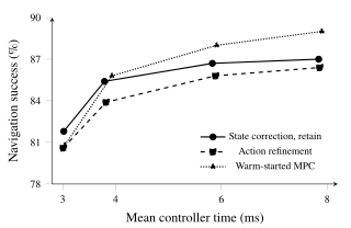
At about 3 ms mean controller time, retained state reaches 81.8% navigation success versus 80.8% for warm-started model predictive control (MPC), which reuses its previous plan to initialize the next optimization. At about 8 ms, MPC reaches 89.0% versus retention's 87.0%.

Within the 4 ms envelope, MPC and retention have similar success, 85.8% versus 85.4%, but MPC has fewer contacts: 6.0 versus 14.2 per 1,000 decisions. A contact is a decision with a physical collision against a wall or obstacle. Our objective penalizes small clearance; MPC and the filters also impose predicted-clearance constraints.

Navigation success across mean controller time budgets. Retained state correction has a higher estimate near 3 ms; warm-started MPC has the higher estimate near 8 ms. — Paper Figure 3. Each point shows a configuration selected on validation data and timed on the same CPU/GPU workstation. View figure ↗

The filters prioritize avoiding contact. The control barrier function (CBF) filter adjusts the next action using a local clearance condition; the predictive filter checks a sequence of actions ahead.

Controller comparisons and timing

Navigation within the 4 ms mean / 8 ms 99th-percentile validation envelope. Paper Table 2. Five independently trained models; ± is the rounded 95% interval half-width.
Controller	Success (%)	Contacts / 1,000 decisions	Mean time (ms)
Frozen recurrent policy	68.4 ± 1.9	37.1 ± 2.3	2.10
CBF filter	79.2 ± 1.6	6.4 ± 0.8	2.58
Predictive filter	82.1 ± 1.5	4.1 ± 0.6	3.92
Action refinement	83.9 ± 1.4	15.9 ± 1.1	3.82
Action + state fitting	85.2 ± 1.3	14.4 ± 1.1	3.91
State correction, discard	82.7 ± 1.5	18.2 ± 1.2	3.81
State correction, retain	85.4 ± 1.3	14.2 ± 1.0	3.79
Warm-started MPC	85.8 ± 1.3	6.0 ± 0.7	3.93

The paired retain-minus-discard success gains are 2.7 percentage points [1.7, 3.7] in navigation and 4.4 [3.1, 5.7] in chain control, with 95% intervals.

Neural inference and derivatives run on an NVIDIA A100; MPC and predictive filtering use one CPU solver thread on the same workstation. Timing includes transfers, failed candidates, cache checks and synchronization.

Sections 5.3 and 5.4; Figure 3; Tables 2 and 3 ↗

Method

The controller proposes a state, then decodes a short action sequence. A local optimizer searches for a nearby state whose decoded plan improves the task objective. Its candidate trials use the same dynamics, residuals and physical limits as direct action refinement.

The correction changes the controller's runtime memory. Its next recurrence starts from the edited state:

\begin{aligned} z_t^\star&=\operatorname{Correct}(z_t^0),\\ z_{t+1}^0&=f_\theta(z_t^\star,x_{t+1}). \end{aligned}

Here \(z_t^0\) is the state before correction, \(z_t^\star\) the retained state, and \(x_{t+1}\) the next observation. The network weights stay fixed.

Decode the current state and evaluate its objective.
Try a correction within the state-displacement limit.
Keep it if the decoded plan passes the action bound and decrease test. Otherwise halve the step and retry.

The optimizer, bounds and decrease test

\(R_t(z)\) combines task errors with a penalty for moving away from the original plan. Its Jacobian \(J\) contains their derivatives with respect to state. A damped Gauss-Newton update gives the search direction:

\begin{aligned} P&=J^\top J+\lambda I,\\ v&=-P^{-1}J^\top R_t(z),\\ z'&=z+\alpha v. \end{aligned}

Damping \(\lambda\) stabilizes the direction. The step size \(\alpha\) controls how far the candidate moves. We accept a candidate only if its evaluated loss decreases and its state and action changes stay within the cumulative bounds.

The reference configuration allows three candidate trials per decision. Rejected candidates consume a trial and reuse the current direction. After acceptance, a remaining trial may compute a fresh direction.

The recurrence proposes \(z_t^0\), and the decoder maps it to a control sequence. The state-search objective includes both task residuals and a proximity term around the initial plan:

\begin{aligned} z_t^0&=f_\theta(z_{t-1},x_t),\\ U_t^0&=g_\phi(z_t^0;c_t),\\ L_t(z)&=F_t\bigl(g_\phi(z;c_t)\bigr). \end{aligned}

The proximity term is part of \(F_t\):

\begin{aligned} F_t(U)&=C_t(U)\\ &\quad+\frac{\mu}{2m}\|S(U-U_t^0)\|_2^2. \end{aligned}

\(C_t\) is the task loss, \(\mu\) sets the proximity weight, \(m\) counts scalar controls, and \(S\) scales them by their physical limits.

Every candidate is checked against the same cumulative bounds around the original proposal:

\begin{aligned} \|z-z_t^0\|_2&\leq\rho_z,\\ \frac{\|S(U-U_t^0)\|_2}{\sqrt m}&\leq\rho_U. \end{aligned}

With \(b=J^\top R_t(z)\), the Armijo acceptance test is:

L_t(z)-L_t(z')\geq-\eta\alpha b^\top v>\epsilon_t.

Non-finite candidates stop the solve. Accepted updates decrease the supplied local objective and remain inside the state ball.

Solving through the output space

The controller has a 256-dimensional state, but its decoded action sequence has 24 dimensions in navigation and 96 in chain control. The exact current-metric solve uses this smaller output space.

Let \(D\) be the decoder Jacobian, \(Q\) the residual Jacobian in action coordinates, and \(A=(Q^\top Q)^{1/2}D\). Then \(P=\lambda I+A^\top A\). The inverse-vector product can be computed as:

\begin{aligned} (\lambda I+AA^\top)q&=Ab,\\ P^{-1}b&=\lambda^{-1}(b-A^\top q). \end{aligned}

The inner system is solved by Cholesky factorization. Derivative and factorization work are included in the reported timing.

Section 2; Algorithm 1; Appendix A ↗

Rollback

A correction can outlive the conditions that made it useful. Changing the target or delaying sensor records removes the average benefit of retention in these tasks. Keeping the original state for one more decision lets the controller withdraw its latest correction.

The simulator supplies a target identifier and sensor-record age. When this metadata shows a changed target or a record more than one decision old, the controller rolls back before its next recurrent update.

Success during intermittent sensing delays (%). Paired gains are percentage points with 95% intervals; paper Table 4.
Task	Always retain	Rollback	Paired gain
Navigation	82.1	83.4	+1.3 [0.5, 2.1]
Chain control	71.8	73.0	+1.2 [0.4, 2.0]

Rollback adds at most 0.02 ms to mean controller time and stays within the same latency limits.

The rollback rule

\begin{aligned} \widehat z_t&=z_t^0+a_{t+1}(\widetilde z_t-z_t^0),\\ a_{t+1}&\in\{0,1\}. \end{aligned}

A zero switch restores the original state; a switch of one keeps the correction. Older changes have already propagated through memory. The action that was executed stays the same.

Paper Section 5.5 and Table 4 ↗

Limits

The study covers one gated recurrent architecture and two simulators with differentiable geometry. It measures what retaining a correction adds within that controller; there is no attention-based baseline.

With stale sensing, the optimizer works from outdated geometry: its supplied objective can improve while physical control deteriorates. Under continuous two-decision observation delay, navigation success falls to 70.4% with retention and 70.9% with discard.

Contact avoidance is a separate limitation: MPC and the filters have much lower contact rates. Rollback also relies on explicit context metadata and only withdraws the latest correction, leaving older changes in recurrent memory.

Outlook

The next comparison is architectural: does a correction leave a similar trace in a state-space model, or in a transformer's key-value cache? Repeating the same paired experiment would measure how long the benefit survives, how much optimizer work it saves, and what can be withdrawn when the context changes.